
Power Integrity and Decoupling Caps
Why Power Integrity?
I hope that you’ve heard about Signal Integrity (SI)— where you engineer the PCB to intentionally control the quality of the signals. This includes the use of termination resistors, controlling trace impedance, and many other techniques.
Power Integrity (PI) is engineering the PCB to intentionally maximize the quality of the power distribution network (PDN). Basically, getting the highest quality power to the places that need it the most.
Let’s be honest here. Most PCB’s are designed with little attention to PI and they work fine, so why should you pay attention to it now? It is only a matter of time before you see problems caused by poor PI. You might even be seeing those problems now but not associating them with PI.
Worst case, you will see failures due to bad PI. Mostly random crashes. At the core, the Apple Intentional Slowdown fiasco is poor PI blamed on poor battery aging but the truth is much more involved. Getting PI correct for Intel based motherboards is so involved that Intel has created special hardware for testing that PI and the PDN meets their specifications.
Even in the best case, you will see problems from poor PI. Increased EMI radiation and susceptibility are the two biggest ones. Not so obvious ones are increased jitter on high speed signaling lines (PCIe, USB, SATA, Ethernet, etc.), bad SI (crosstalk like issues), and lower overall design margin.
Engineers are most likely to first experience bad PI at the EMC test lab. But a significant number first run into it when they start to get complains and returns from customers in the field. This can be a huge problem, and quite a few product recalls are due to bad PI!
DC Analysis
It is helpful to look at this from a DC point of view first, and then go to the slightly more complicated AC analysis.
Most power rails for chips have some sort of tolerance requirement on them. For example, a 1.8v rail is required to be accurate withing 5%. That gives you a voltage range of 1.71 to 1.89 to play in. From that range, we subtract all sorts of things like noise and tolerances. Whatever remains of that range is your design margin. You want that margin to be as large as possible for the most reliable product.
Tolerances are not the focus of this article, but I want to briefly mention them. Voltage regulators are not perfect, and have variation from their nominal feedback voltage. The resistors you use to set the output voltage also have a tolerance. These tolerances can stack up, and if you don’t pay attention to them could create a problem. Even using 1% resistors, these inaccuracies could eat up 3% or more of your 5% requirement— leaving little or no margin. Don’t ignore tolerances in your voltage regulators.
Ripple (and noise in general) also eat into your margin, but what we are most interested in is voltage drop due to power rail impedance.
For our DC analysis you can think of rail impedance as ESR. Let’s say that your processor draws 10 amps on a 1 volt rail. Let’s also say that your power rail impedance is 0.01 ohms. This means, according to ohms law, that you will see a 0.1 volt drop, or 0.9 volts at the CPU. That is very outside of the 5% requirement of the CPU!
Moving to AC
When we start thinking of this in the frequency domain, things get interesting. Instead of considering the static load on the power rail, we consider transient loads. Transients are caused by circuits doing something. So any useful circuit has transients. In digital circuits they are most often caused by signals transitioning between low and high.
The magnitude of the transient can vary greatly, and can be hard to predict. The worst offender are wide parallel busses that have all the outputs changing at the same time. DDR memory or parallel flash is a good example of this.
A low-end Intel CPU can have massive transients. One particular model lists 20 amp transients in the datasheet! A 20 amp transient load on our previous example of 0.01 ohms impedance would put our 1.0 volt rail at 0.8 volts! That’s horrible.
It is important to remember that the repetition rate of a signal is not the same as the frequency content of the signal. There are harmonics to consider. A 100 MHz clock, for example, has a lot of odd-harmonics. If you looked at a spectrum analysis of it, you will see 300 MHz, 500 MHz, etc. On up to infinity. Well, in theory it goes up to infinity but in reality it maybe goes up a little past 1 GHz. Most of the energy will be at the fundamental frequency (100 MHz), and the energy levels go down as the frequency goes up.
The power rail impedance varies over frequency. It might be very low in one spot, but very high in another. If your load has a frequency component that lines up with a high spot in the impedance then you will have unusually high noise at that frequency.
Target Impedance
Your target impedance is calculated like ohms law. The formula is this:
Allowable Voltage Swing = Power Rail Impedance * Maximum Transient Current
The problem with this formula is that the maximum transient current is often not know, and it is difficult to measure. But it does give you a good place to start.
If not known, a target power rail impedance of 0.01 ohms is a good place to start.
This is not a hard and fast rule. 0.01 ohms is fine for many applications, but simple boards might get away with a higher value and more demanding boards need to be lower.
For now, assume that your target impedance is even across the whole frequency range. So if it is 0.01 ohms at 1 MHz, it is also 0.01 ohms at 1 GHz. There are times that doesn’t have to be flat, but that’s beyond the scope of this article.
Another factor for your target impedance is any noise requirements. It is possible that you could have sufficient noise on a power rail to disrupt operation, but still have the voltage remain within the min/max specified in the IC datasheet. If this is an issue, then your target impedance needs to be low enough to minimize this noise.
But Not Too Low
The target impedance is a target to get close to. Not a maximum that you must stay below.
The reason why is very complex and too involved for this article. I will try to cover this topic in a future article. But the quick answer is that the PDN is full of parallel and series resonances. An unusually low impedance encourages those resonances to be worse than we would like. Keeping the impedance low, but not too low, keeps a lot of that under control.
What Controls PDN Impedance
Capacitors. Under about 10 KHz, impedance is controlled by the voltage regulators. Above that, it is almost entirely controlled by capacitors. Here is a rough guide to what frequencies are controlled by what:
<10 KHz: The voltage regulator itself.
10 KHz – 400 KHz: Large output caps of the voltage regulator, usually electrolytic.
400 KHz – 1 MHz: Bulk ceramic caps (1 uF to 22 uF).
1 MHz to 250 MHz: Ceramic decoupling caps (1 nF to 1 uF).
>250 MHz: Embedded capacitance made by having power and ground planes placed close together in the PCB.
Parasitics (ESR and ESL) of the caps matter a lot, as does the PCB layout.
Decoupling Caps
In The Nature of Capacitors Part 1 and Part 2, I discussed the important features of capacitors and how to simulate them.
Download the LTspice simulation for this article here.
The graph below shows the combined impedance of 88 decoupling capacitors of different values, working toward a target impedance of 0.01 ohms.
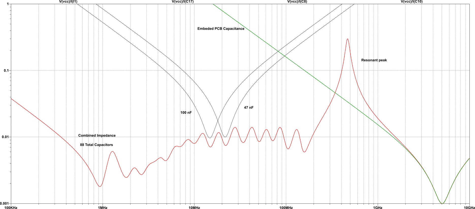
Shown for amusement sake are the individual contributions of the three 100 nF caps, four 47 nF caps, and the embedded PCB capacitance. No large bulk caps or regulator output caps were included, hence why the impedance rises below 1 MHz.
Another important feature of the graph is the large resonant peak at 470 MHz. This peak is caused by the parallel resonance of the embedded capacitance and the parasitic inductance of the other capacitors. This peak will be covered in a future blog article; but for now know that it is hard to get rid of, is extremely dependent on all of the parasitics on the PCB, and almost impossible to simulate accurately in advance. The usual way to handle it is try to minimize it in simulations as best you can, but measure and tweak things once the PCB has been built. Yes, this is an ugly one but it also looks much worse than it really is.
Eighty-eight capacitors sounds like a lot, but it is about typical for many boards and a small number for a lot of them. The exact number of caps can be varied depending on the demands of the actual PCB. There are also 14 different cap values used, which could be varied as well.
In the PI_PDN simulation included in the Zip file for this blog post, you can see and vary the caps. If you used this as the starting point for designing your own PDN, you would want to change not just the cap value and quantity, but also the ESL, ESR, and fanout inductance. I chose those values to be representative of what you might use, but it is almost certainly wrong for the parts you use.
How About Less Cap Values?
Some people advocate using a single capacitor value, or maybe three different values— but there is a problem with that approach.
Earlier I said that your target impedance is a target, not a maximum. The ideal shape of the impedance curve would be a flat line. We use many cap values to help us approximate that flat line as best we can.
Using a single, or even three, cap values creates an impedance graph where the deviations from our ideal impedance is too great. Either too high, creating a potential for noise, or too low creating the potential for bad resonances to develop elsewhere.
Decoupling Capacitor Rules Of Thumb
If you do a Google search for “decoupling capacitor rule of thumb” you will see many rules. The vast majority of them are wrong.
Any rule of thumb that doesn’t factor in your target impedance, operating frequencies, and noise margins cannot hope to be correct. Like most rules, they are valuable when we are too immature to understand the correct reasoning, but we should quickly outgrow them in favor of a more informed and intentional approach.
Conclusion
Getting the decoupling caps correct is difficult, and often seems more like art than science. It doesn’t help that there is a lot of misinformation out there on the Internet and in books. But understanding what the goal of decoupling caps is, and knowing how to simulate them, is a huge step in getting it more correct.